2. MDP

Really useful link for learning RL and Game theory

Markov Decision Process

The Bellman Equation

$$V(s) = \max_{a \in A(s)} \sum_{s' \in S} P_a(s'|s) [r(s, a, s') + \gamma V(s')]$$

• $\gamma$ : discount factor
• $P_a(s'|s)$ : transition probability
• $r(s, a, s')$ : reward

Policy Extraction : DECIDING HOW TO ACT

$$\pi(s) = \arg \max_{a \in A(s)} \sum_{s' \in S} P_a(s'|s) [r(s, a, s') + \gamma V(s')]$$

(提取最优action)

The multi-armed bandit problem

A mukti-armed bandit (also known as an N-armded bandit) is defined by a set of random variables $X_{i,k}$ where:

• $1 \leq i \leq N$ such that $i$ is the arm of the bandit; and
• k the index of the play of arm $i$

The idea is that a gambler iteratively plays rounds, obervaing the reward from the arm after each round, and can adjust their strategy each time. The aim is to maximize the sum of the rewards collected over all rounds.

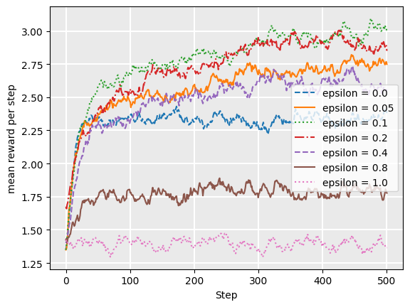
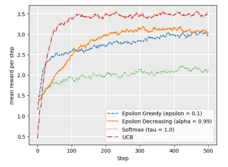
$\epsilon$-greedy stragegy

• With probability $1-\epsilon$ wo choose the arm with maximum Q value $\argmax_a Q(a)$ (exploit).
• With brobability $\epsilon$ we choose a random arm with uniform probability (explore)

Softmax strategy

$$\frac{e^{Q(s, a) / \tau}}{\sum_{b=1}^{n} e^{Q(s, b) / \tau}}$$

Softmax is a probability matching strategy, which means that the probability of each action being chosen is dependent on its Q-value so far.

UCB1 (upper condifence bounds) Using the UCB1 strategy, we select the next action using the following:

$$\argmax_a \left( Q(a)+ \sqrt{\frac{2 \ln t}{N(a)}} \right )$$

where $t$ is the number of rounds so far, and $N(a)$ is the number of times $a$ has been chosen in all previous arounds.

• The left term encoueages exploitation: the Q-value is high for actions that have had a high reward
• The right term encourages exploration: it is high for actions that have been explored less, that is, when $N(a)$ relative to other actions. As $t$ increases, if some actions have low $N(a)$, then the expression $\sqrt{\frac{2 \ln t}{N(a)}}$ is large compared to actions with higher $N(a)$

Model-based vs model-free

Value iteration is part of a class of solutions known as model-based techniques. This means that we need to know the model, in particular, we have access to $P_a(s'|s)$ and $r(s, a, s')$.

How can we calculate a policy if we don't know the transitions and rewards? we learn through experience by trying actions and seeing what the result is, making this machine learning problem. We learn a value function or a policy directly.

Temporal-difference learning

Model-free reinforcement learning is learning a policy directly from experience and rewards. Q-learning and SARSA are two model-free approaches.

$$Q(s, a) \leftarrow Q(s, a) + \alpha [r + \gamma V(s') - Q(s, a)]$$

• $\alpha$: Learning rate
• $r$: Reward
• $\gamma$: discount factor

Q-learning: Off-policy temporal difference learning

$V(s') \leftarrow \max{(Q(s', a'))}$

SARSA: On-policy temporal difference learning

$V(s') \leftarrow Q^{\pi}(s', a')$

Q-learning vs SARSA

• Q-Learning
  • Q-learning will converge to the optimal policy
  • But it can be 'unsafe' or risky during training.
• SARSA
  • SARSA learns the safe policy, mayve not that optimal.
  • SARSA receibes a higher average reward via training.

The difference between SARSA and Q-learning is that Q-learning is off-policy learning, while Sarsa is on-policy learning. Essentially, this means that SARSA chooses its action using the same policy used to choose the previous action, and then uses this difference to update its Q-function; while Q-learning updated assuming that the next action would be the action with the maximum Q-value.

Q-learning is therefore "optimistic", in that when it updates, it assumes that in the next state, the greedy action will be chosen, even it may be that in the next step, the policy, such as $\epsilon$-greedy, will choose to explore an action other than the best.

SARSA instead knows the action that it will execute next when it performs the update, so will learn on the action whether it is best or not.

On-policy vs. off-policy: Why do we have both?

The main advantage of off-policy approaches is that they can use samples from sources other than their own policy. For example, off-policy agents can be given a set of episodes of behaviour from another agent, such as a human expert, and can learn a policy by demonstration.

n-step SARSA

$$G_t^n = r_t+\gamma \cdot r_{t+1} + \gamma^2 \cdot r_{t+2}+\dots +\gamma^n \cdot Q(s',a') \\[6pt] Q(s_t, a_t) \leftarrow Q(s_t, a_t) + \alpha [G_t^n - Q(s_t, a_t)]$$

Shape reward

$$Q(s, a) \leftarrow Q(s, a) + \alpha \left[ r + \underbrace{F(s, s')}_{\text{additional reward}} + \gamma \max_{a'} Q(s', a') - Q(s, a) \right]$$

The purpose of the function is to given an additional reward $F(s, s')$ when any action transitions from state $s$ to $s'$. The function: $F$ providees heuristic domain knowledge to the problem that is typically manually programmed.

Potential based Reward Shaping

$$F(s,s') = \gamma \Phi(s') - \Phi(s)$$

$\Phi(s)$ is the potential of state $s$.
Important : discount factor $\gamma$ on $\Phi(s')$

Linear Q-function Arroximation

The key idea is to approximate the Q-function using a linear combination of features and their weights. Instead of recording everything in detail.

The overall process:

1. for the states, consider what are the features that dettermine its representation;
2. during learning, perform updates based on the weights of features indtead of states; and
3. estimate $Q(s,a)$ by summing the features and their weights.

Rrepresentation

1. A feature vector, $f(s,a)$ which is a vector of $n \cdot |A|$ different features, where $n$ is the number of features and $|A|$ is the number of actions.

It is straightforward to construct $n \times |A|$ state pair features from just $n$ state features.

$$f_{i,k}(s,a) = \begin{cases} f_i(s) & \text{if } a = a_k \\ 0 & \text{otherwise} \quad 1 \leq i \leq n, 1 \leq k \leq |A| \end{cases}$$

This effectively results in $|A|$ different weight vectors:

$$f(s,a_1) = \begin{pmatrix} f_{1,a_1}(s,a) \\ f_{2,a_1}(s,a) \\ 0 \\ 0 \\ 0 \\ 0 \\ \vdots \end{pmatrix} f(s,a_2) = \begin{pmatrix} 0 \\ 0 \\ f_{1,a_2}(s,a) \\ f_{2,a_2}(s,a) \\ 0 \\ 0 \\ \vdots \end{pmatrix} f(s,a_3) = \begin{pmatrix} 0 \\ 0 \\ 0 \\ 0 \\ f_{1,a_3}(s,a) \\ f_{2,a_3}(s,a) \\ \vdots \end{pmatrix} \ldots$$

2. A weight vector $w$ of size $n \times |A|$: One weight for each feature-action pair. $w_{i}^{a} defines the weight of a feature$i$for action$a$.

Q-values from linear Q-function

Given a feature vector $f$ and a weight vector $w$, the Q-value of a state is a linear combinations of features and weights.

$$Q(s,a) = f_1(s,a) \cdot w_1^a + f_2(s,a) \cdot w_2^a + \ldots + f_n(s,a) \cdot w_n^a \\ = \sum_{i=0}^n f_i(s,a)w_i^a$$

Linear Q-function update

$$w_i^a \leftarrow w_i^a + \alpha[r + \gamma \max_{a'} Q(s', a') - Q(s,a)]f_i(s,a)$$

$\max_{a'} Q(s', a')$ can be altered depand on the algorthm used.

• A action only updates the weights corresponded to the features of the action.

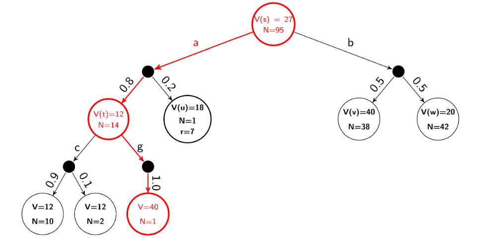
Monte Carlo Tree Search

Value updation for expectimax tree

$$V(t) = \max_{a' \in \{c, g\}} \sum_{t' \in \text{children}(t)} P_{a}(t' \mid t) \left[r(t, a', t') + \gamma V(s(t'))\right]$$