Part of Speech Tagging

What is a POS tagging?

• a label assigned to a word in a sentence indicate its grammatical role.

Assumptions that go into a Hidden Markov Model

• Markov assumption: The current state (POS tag) depends only on the previous state.
• Output independence：The obserced word depends only on the current state(tag), not on other words or states.
• Stationary Transition and emission probabilities do not change over time.

Time complexity of the Viterbi algorithm

$O(T \times N^2)$ where: T = length of the sequence (number of words) N = number of possible tags

Its practical for POS tagging since the number of tags (N) is small (N $\lt$ 50 for most languages)

Example

Answer

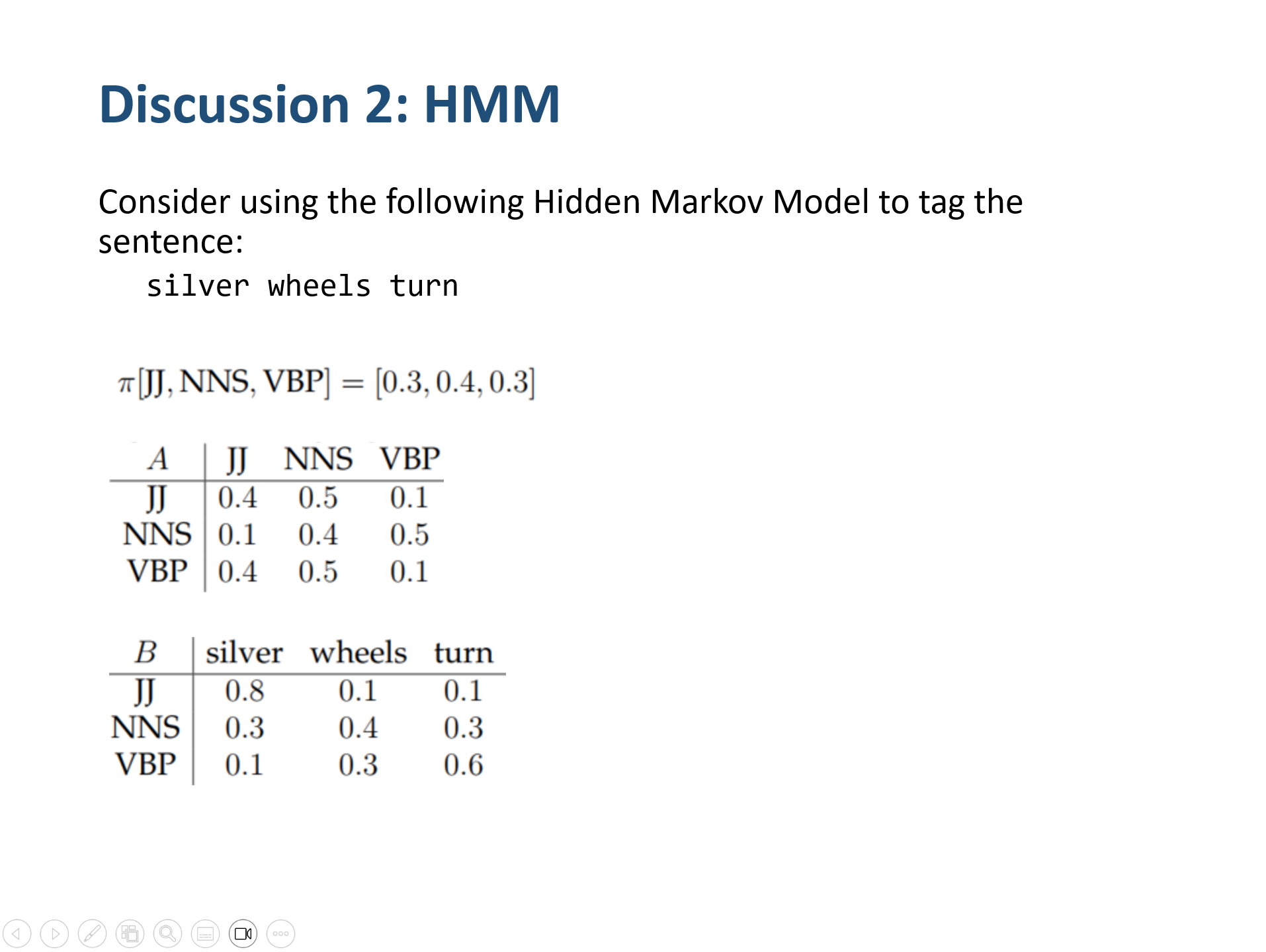
Initial state distribution:

$$\pi(\text{JJ})=0.3,\quad \pi(\text{NNS})=0.4,\quad \pi(\text{VBP})=0.3$$

The transition probability matrix:

$$A=\begin{pmatrix} p(\text{JJ}\to\text{JJ}) & p(\text{JJ}\to\text{NNS}) & p(\text{JJ}\to\text{VBP})\\[5mm] p(\text{NNS}\to\text{JJ}) & p(\text{NNS}\to\text{NNS}) & p(\text{NNS}\to\text{VBP})\\[5mm] p(\text{VBP}\to\text{JJ}) & p(\text{VBP}\to\text{NNS}) & p(\text{VBP}\to\text{VBP}) \end{pmatrix} = \begin{pmatrix} 0.4 & 0.5 & 0.1\\[3mm] 0.1 & 0.4 & 0.5\\[3mm] 0.4 & 0.5 & 0.1 \end{pmatrix}$$

The emission probability matrix (with the observed vocabulary $\{ \text{silver, wheels, turn}\}$) is：

$$\begin{aligned} &p(\text{silver}|\text{JJ})=0.8,\quad p(\text{wheels}|\text{JJ})=0.1,\quad p(\text{turn}|\text{JJ})=0.1,\\[5mm] &p(\text{silver}|\text{NNS})=0.3,\quad p(\text{wheels}|\text{NNS})=0.4,\quad p(\text{turn}|\text{NNS})=0.3,\\[5mm] &p(\text{silver}|\text{VBP})=0.1,\quad p(\text{wheels}|\text{VBP})=0.3,\quad p(\text{turn}|\text{VBP})=0.6. \end{aligned}$$

Viterbi Algorithm for “silver wheels turn”

Let the observation sequence be

$$O = (\text{silver}, \text{wheels}, \text{turn}),$$

and let the hidden state sequence be

$$(s_1, s_2, s_3) \in \{\text{JJ}, \text{NNS}, \text{VBP}\}^3.$$

Initialization ($t=1$, word “silver”)

$$\begin{align} \delta_1(\text{JJ}) &= \pi(\text{JJ}) \times p(\text{silver}|\text{JJ}) = 0.3 \times 0.8 = 0.24,\\[1ex] \delta_1(\text{NNS}) &= \pi(\text{NNS}) \times p(\text{silver}|\text{NNS}) = 0.4 \times 0.3 = 0.12,\\[1ex] \delta_1(\text{VBP}) &= \pi(\text{VBP}) \times p(\text{silver}|\text{VBP}) = 0.3 \times 0.1 = 0.03. \end{align}$$

Step 2: Recursion ($t=2$, word “wheels”)

$$\delta_2(s) = \max_{s'\in\{\text{JJ, NNS, VBP}\}} \left[\delta_1(s') \times p(s' \to s)\right] \times p(\text{wheels}|s).$$

1. $\delta_2(JJ)$

$$\begin{align} &\delta_1(JJ) \times p(JJ \rightarrow JJ) \times p(\text{wheels}|\text{JJ}) = 0.24 \times 0.4 \times 0.1 = 0.0096 \\[1ex] &\delta_1(NNS) \times p(NNS \rightarrow JJ) \times p(\text{wheels}| JJ) = 0.12 \times 0.1 \times 0.1 = 0.0012 \\[1ex] &\delta_1(VBP) \times p(VBP \rightarrow JJ) \times p(\text{wheels} | JJ) = 0.03 \times 0.4 \times 0.1 = 0.0012 \\[1ex] \end{align}$$

Choose the max value 0.0096, from $JJ \rightarrow JJ$

$\delta_2(JJ) = 0.0096$

2. $\delta_2(NNS)$

$$\begin{align} &0.24 \times 0.5 \times 0.4 = 0.048 \\ &0.12 \times 0.4 \times 0.4 = 0.0192 \\ &0.03 \times 0.1 \times0.4 = 0.006 \\ \end{align}$$

Choose the max value 0.048 , from $JJ \rightarrow NNS$

$\delta_2(NNS) = 0.048$

3. $\delta_2(VBP)$

$$\begin{align} &0.024 \times 0.1 \times 0.3 = 0.0072 \\ &0.12 \times 0.5 \times 0.3 = 0.018 \\ &0.03 \times 0.1 \times 0.3 = 0.0009 \\ \end{align}$$

Choose max Value 0.072, from $NNS \rightarrow VBP$

Step 3: Recursion ($t=3$, word “sliver”)

Same as previous one

$$\delta_3(s) = \max_{s'\in\{\text{JJ, NNS, VBP}\}} \left[\delta_2(s') \times p(s' \to s)\right] \times p(\text{turn}|s).$$ $$\begin{align} &\delta_3(JJ) = 0.00072 \\ &\delta_3(NNS) = 0.00576 \\ &\delta_3(VBP) = 0.0144 \\ \end{align}$$

Step 4 Termination and Backtracking

At $t=3$, we compare:

$$\delta_3​(JJ)=0.00072,\quad \delta_3​(NNS)=0.00576,\quad \delta_3​(VBP)=0.0144$$

The highest probability is 0.0144 for state VBP. Backtracking the recorded predecessor states:

• At $t=3$, the best state is VBP.
• At $t=2$, the best transition leading to VBP came from NNS.
• At $t=1$, the best transition leading to NNS came from JJ.

which corresponds to the following tagging:

• silver → JJ
• wheels → NNS
• turn → VBP