FNNs and RNNs
Feedforward Networks
1. Introduction to Feedforward Neural Networks
- Feedforward Neural Networks (FNNs): Also called multilayer perceptrons (MLPs).
- Structure:: Input Hidden Layers Output.
- Neurons:: Each neuron applies weights, adds bias, and passes through a non-linear function (e.g., sigmoid, tanh(hyperbolic sigmoid), ReLU).
2. Mathematical Fromulation
- Single Neuron
- Matrix Notation
3. Output Layer
- Binary Classification: Sigmoid activation
- Multi-class Classification: Softmax activation ensures output probabilities sum to 1.
4. Training and Optimization
- Objective: Maximize likelihood , or minimize loss .
- Optimizer: Gradient Descent (via frameworks like TensorFlow, Pytorch).
- Regularization Techniques
- L1: Sum of absolute values.
- L2 : Sum of squares.
- Random Dropout: Randomly zero-out neurons to prevent overfitting.
5. Applications in NLP
5.1 Topic Classification
-
Input : Bag-of-words or TF-DF
-
Network:
-
Prediction: Class with highest softmax output
5.2 Language Modelling
- Goal : Estimate the probability of word sequences.
- FFNN LM:
- Input = embeddings of previous words (e.g., trigram context).
- Output = next word.
- Uses learned word embeddings to represent input words.
6. Word Embeddings
- Purpose: Map discrete words to continuous vectors.
Recurrent Networks
1. Recurrent Neural Neworks (RNNs)
Core Concepts
- Designed to process sequential data of arbitary length
- Maintians a State vector to capture information from previous time steps.
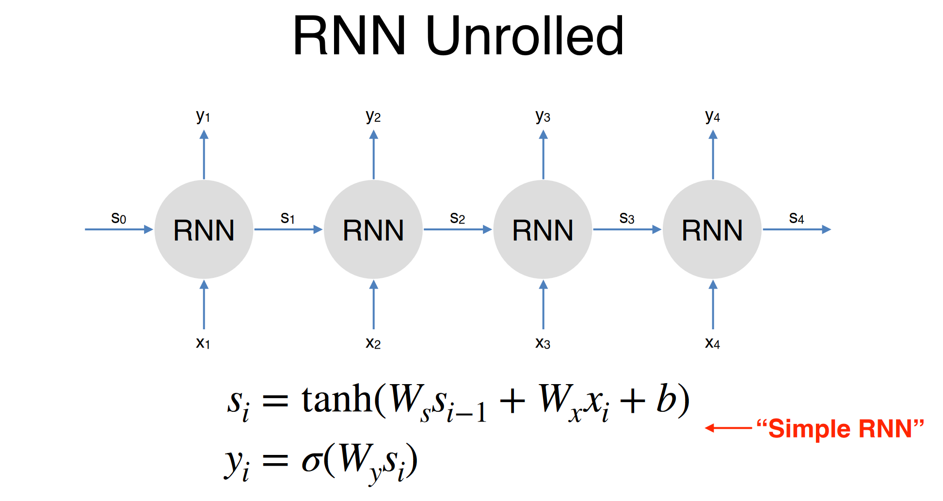
- Process input one token at a time using the Recurrence formula
RNN Architecture
- Unrolled RNN: each time step reuses the same parameter.
- Traning uses Backpropagation Through Time(BPTT)
2. Limitaion of RNNs
- Difficulty capturing long-range dependencies due to vanishing gradients
- Performance degrades when trying to model long contexts.
3. Long Short-Term Memory (LSTM)
3.1 Motivation
- Designed to overcome vanishing gradient problems in RNNs.
3.2 Components
- Memory cell: stores long-term information
- Gates: control the flow of information:
| Aspect | RNN | LSTM |
|---|---|---|
| Long-term memory | ❌ Poor | ✅ Good with gating mechanism |
| Training speed | ✅ Faster | ❌ Slower due to more computation |
| Expressiveness | ✅ Flexible | ✅ Even more expressive |
| Popularity | 🔻 Declining | 🔻 Replaced by Transformers in SOTA |