Transformer and Word Embedding

Transformer and Attention

1.Background and motivation

1.1 RNN Limitations

In traditional Recurrent Neural Networks (RNN) or LSTM models, the sequence is processed one token at a time: the $t$-th token connot be processed until $(t-1)$-th token is finished. This captures sequential information but leads to 2 major drawbacks:

1. Non-parallelizable: Slow training speed.
2. Long-range dependency problem: It becomes difficult for RNNs to propagate information from distant positions in the sequence effectively.

1.2 The Emgergence of the Transformer

In 2017, Vaswani et al. introduced the Transformer architecture in the paper Attention is All You Need, revolutionizing Natural Language Processing (NLP) and deep learning. The key innovation in the Transformer is the Self-Attention Mechanism, which captures dependencies across all positions in a sequence In parallel, without relying on recurrent structures.

2. Fundamentals of Attention

2.1 Concept of Attention

The core idea of Attention is that when the model focuses on a particular target word (or position), it should "attend" to the most relevant parts of the input sequence, assigning higher weights to those relevant elements.

• A simple analogy: When we read, we tent to focus more on words or sentences most relevant to the question at hand.

2.2 The introduction of Query, Key， and Value

Practically, each token is projected into three different vector spaces:

• Query (Q): "What am I looking for?
• Key (K): "What features do I have for retrival?"
• Value (V) "What content do I actually carry?"

In Self-Attention, every token in the sequence serves as a Query, Key, Value. Each token compares itself to others, resulting in distinct attention weights.

3. Self-Attention Formula Derivation

3.1 Basic From

The most common form is Scaled Dot-Product Attention. The core formula is:

$$\text{Attention}(Q,K,V) = \text{softmax}(\frac{Q K^T}{\sqrt{d_k}})V$$

• $Q\in \mathbb{R}^{n \times d_k}$：Matrix containing all Query vectors (where $n$ is the sequence length, and $d_k$ is the dimension of each vector)
• $K \in \mathbb{R}^{n \times d_k}$: Matrix containing all Key vectors
• $V \in \mathbb{R}^{n \times d_v}$: Matrix cotaining all Value vectors (often $d_v$ = $d_k$)
• $QK^T \in \mathbb{R} ^{n \times n}$： Computes pairwise similarity (dot-product) among tokens.
• $\sqrt{d_k}$: A scaling factor to prevent large dot-product values from destabilizing gradients.

3.2 Step-by-step Derivation

1. Compute similarity scores:

$$\text{Scores} = QK^T$$

This step produces the "matching" degree of each token against all others.

2. Scaling:

$$\text{ScaledScores} = \frac{\text{Scores}}{\sqrt{d_k}}$$

Prevents overly large inner product values, ensuringt gradient stability.

4. Mutl-Head Attention

4.1 Why Muti-Head?

Words in a sentence can relate to each other across multiple dimensions (syntax, semantics, context). A Single attention head may struggle to attend to all these facets simultaneously. Hence, Multi-Head Attention is introduced. Multiple heads perform separate projections and attentions in parallel, and their outputs are concatenated and linearly transfromed, capturing richer relationships.

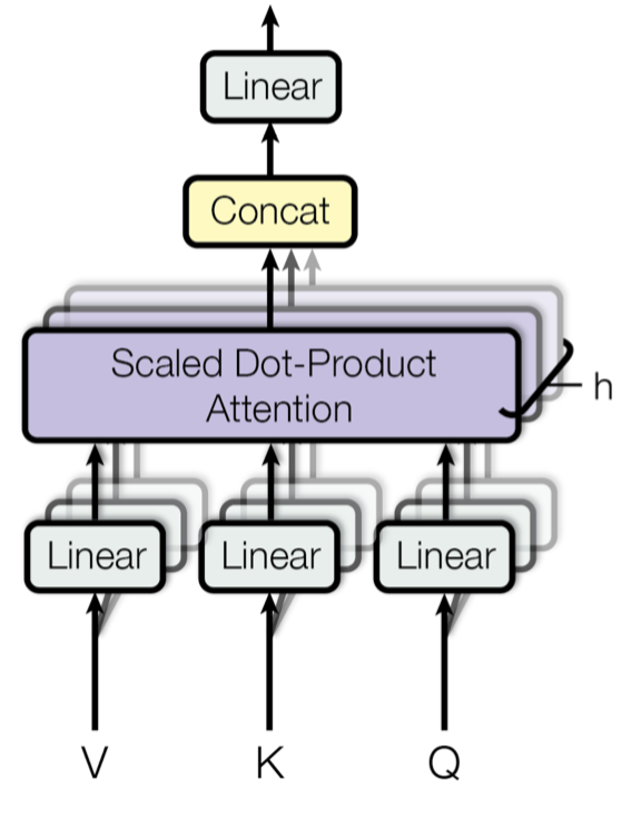
4.2 Multi-Head Formula

Assume we have $h$ attention heads, each with its own projection matrices $W_i^Q$, $W_i^K$, $W_i^V$. The $i$-th head is computed as:

$$\text{head}_i = \text{Attention}(QW_I^Q, KW_I^k, VW_i^V)$$

We then conatenate all $\text{head}_i$ amd multiply by an output projection matrix $W^O$:

$$\text{MultiHead}(Q,K,V) = \text{Concat} (\text{head}_1, \dots, \text{head}_h) W^O$$

5. Transformwer block Structure

6. Word Embedding

6.1 Why Position Emcoding

Self-Attention in a Transformer does not inherently distinguish the positions of tokens in a sequence. Without additional signals, the model cannot tell which token appears first or second. Hence, Postion information must be explictly injected

1. Word Embedding

1.1 Distribution Hypothesis

The distribution hypothesis states, "You shell know a word by the company it keeps." Both locak context (word windows) and document-level co-occurance signal a word's meaning (Firth,1957).

1.2 Guessing Meaning from context

• Learn unknown word from its usage

• Another way： look at words that share similar contexts

1.3 Word vectors

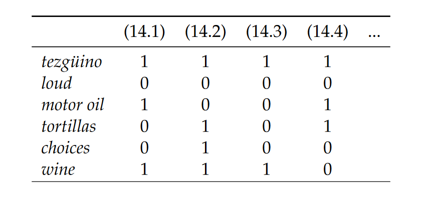
• Each row can be thought of a word vector
• It describes the distributional properties of a word
  • i.e., encodes information about its context words
• Capture all sorts of semantic relationships

Word embeddings

2. Count-Based Word vectors

• Gneneral two flavours
  • Use document as context
  • Use neighbouring words as context

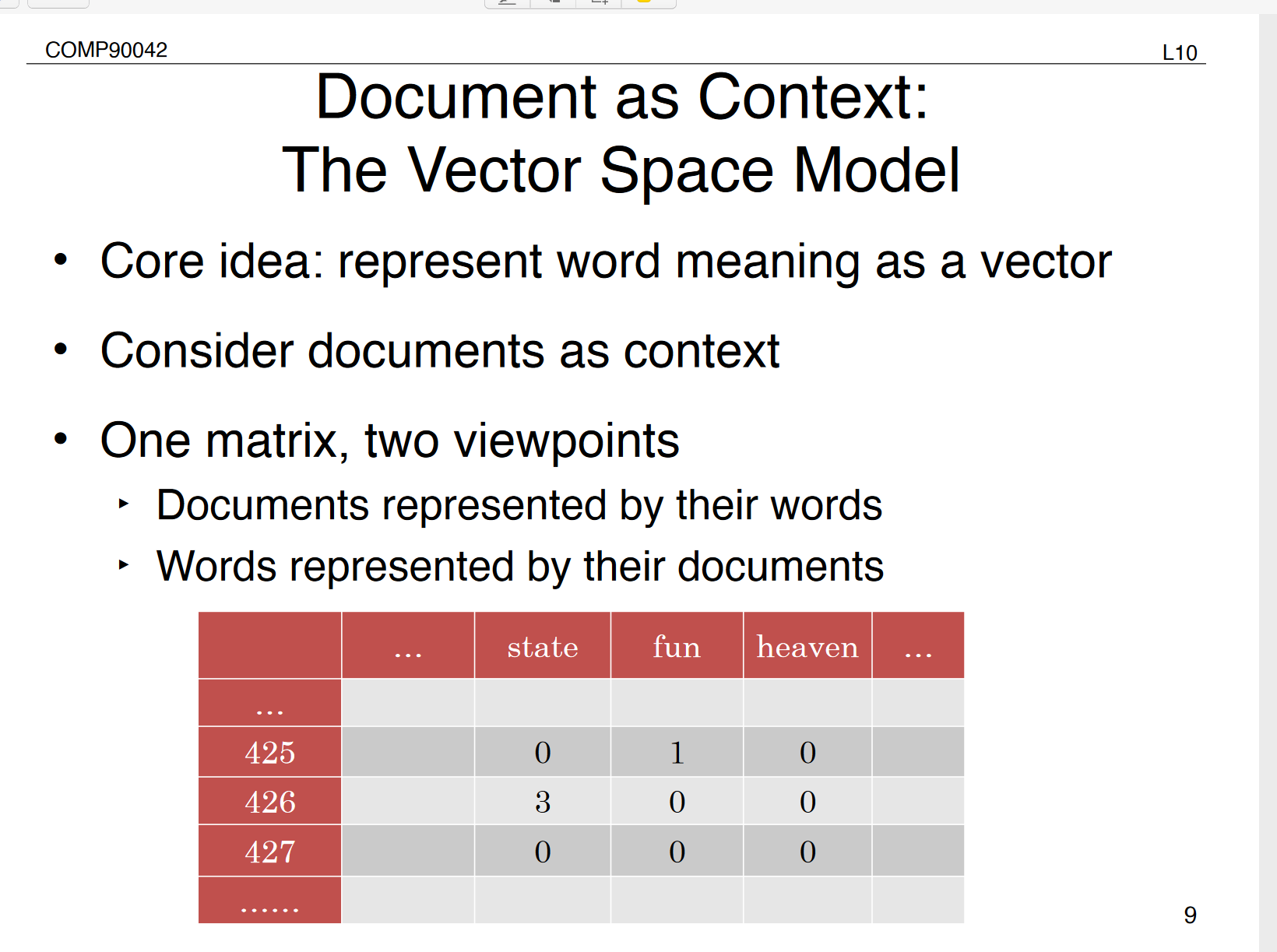
2.1 Docuement as Context: The Vector Space Model

• Core idea: represent word meaning as a vector
• Consider documents as context
• One matrix, two viewpoints
  • Documents represented by their words
  • Words represented by their documents

Manitupulating the VSM:

• Weighing the values (beyond frequency)
• Creating low-dimensional dense vectors

2.2 Tf-idf

$$idf_w = \log{\frac{|D|}{df_w}}$$

where $D$ is total # of docs and $df_W$ is #docs that has w

• Standard weighting scheme for information retrieval
• Discounts common words

2.3 dimensionality Reduction

• Term-document martrices are very sparce
• Dimensionality reduction: create shorter, denser vectors
• More practial (less features)
• Remove noise (less overfitting)

2.4 Singular Value Decomposition

$$A = U \Sigma V^T$$

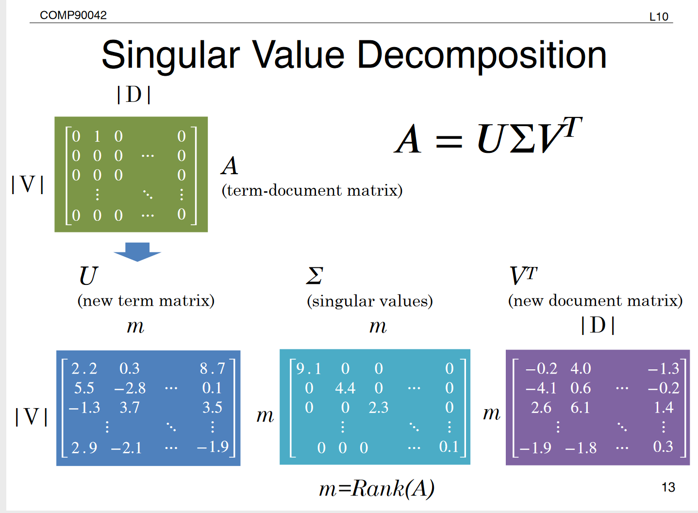
2.4 Truncating - Latent Semantic Analysis

• Truncating $U,\Sigma, V$ to k dimensions produces best possible k rank appriximation of original matrix
• $U_k$ is a new low dimensional representation of words
• Typical values for k are 100-5000

3 Words as Context

• Lists how often words appear with other Words
  • In some predefined context (e.g., a window of N words)
• The obvious problem with raw frequency: dominated by common words

3.1 Pointwise Mutual information

• For two events x and y, PMI comoputes the discrepancy between:
  • Their joint distribution = $P(x,y)$
  • Their individual distributions (assuming independence) = $P(x)P(y)$

$$PMI(x,y) = \log_2\frac{P(x,y)}{P(x)P(y)}$$

PMI primarily serves as a weighted co-occurance matrix, used to measure the strengthj of semantic association between a word w and a contgext word can

3.2 PMI matrix

• PMI does a better job of capturing semantics
  • e.g., heaven and hell
• But very biased towards rare word pairs
• And doesn't handle zeros well

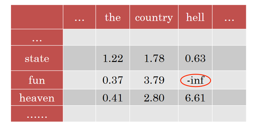
3.3 PMI tricks

• Zero all negative values (Positve PMI)
  • Avoid -inf and unreliable negative values
• Counter bias towads rare events

$$\text{Normalised PMI: }\quad \left( \frac{\text{PMI(x,y)}}{-\log P(x,y)}\right)$$

3.4 SVD (A = $U \Sigma V^T$ )

• Regardless of whatever we use document or word as context, SVD can be applied to create dense vectors

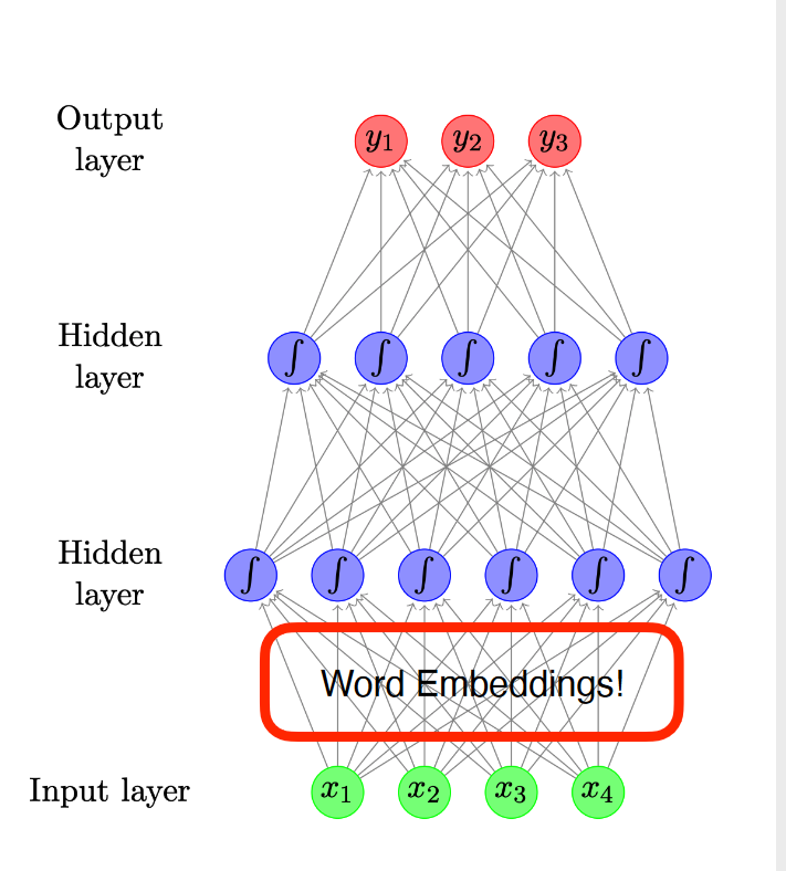
4.Neural Methods

• We've seen word embeddings used in neural neworks (lecture 7 and 8)
• But these models are designed for other tasks:
  • Classcification
  • Languager modeling
• Word embedding are just byproduct

4.1 Word2Vec

Core idea:

• You shall know a word by the company it keeps
• Predict a word using context words

Word2Vec has 2 structures:

• Skip-gram: predict surrounding words of target word

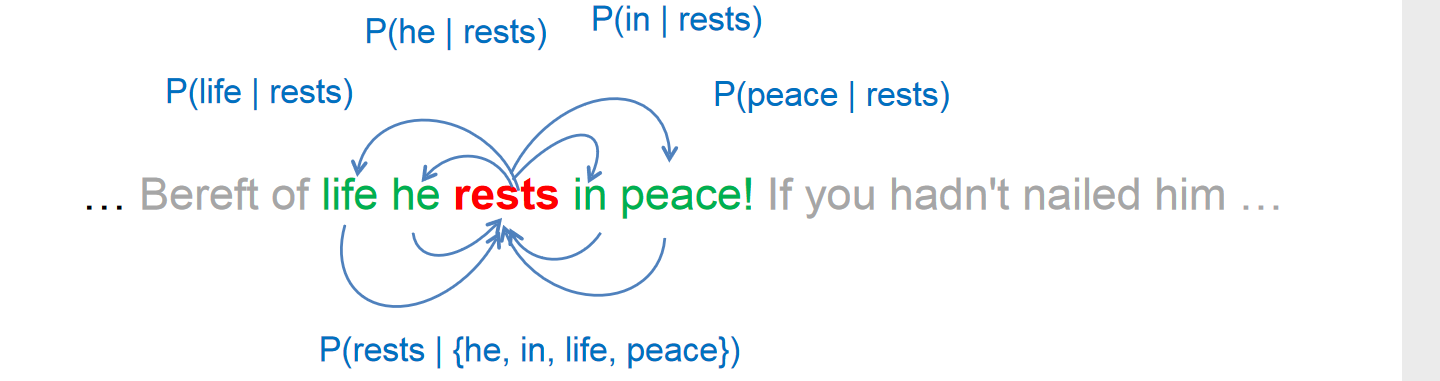
• CBOW: predict target word using surrounding words