Basic computing and quantum computing Theory

Basic Math

Recall that the modulus of a complex number $a + ib$ is given by $| a + ib | = \sqrt{a^2 + b^2}$
and the complex conjugate is given by $\overline{a + ib} = a - ib$.

$| 6 + \pi i | = \sqrt{6^2 + \pi^2}; \quad \overline{6 + \pi i} = 6 - \pi i$

$$\begin{align*} |0\rangle = \begin{bmatrix} 1 \\ 0 \end{bmatrix}; \quad |1\rangle = \begin{bmatrix} 0 \\ 1 \end{bmatrix} \end{align*}$$

Quantum gates:

$$\begin{align*} H = \frac{1}{\sqrt{2}}\begin{bmatrix} 1 & 1 \\ 1 & -1 \end{bmatrix}; \quad T = \begin{bmatrix} 1 & 0 \\ 0 & e^{i\frac{\pi}{4}} \end{bmatrix}; \quad S = \begin{bmatrix} 1 & 0 \\ 0 & i \end{bmatrix} = T^2 \end{align*}$$

Pauli matrices:

$$\begin{align*} \sigma_0 \equiv I \equiv \begin{bmatrix} 1 & 0 \\ 0 & 1 \end{bmatrix} \quad \sigma_1 \equiv \sigma_x \equiv X \equiv \begin{bmatrix} 0 & 1 \\ 1 & 0 \end{bmatrix} \end{align*}$$ $$\begin{align*} \sigma_2 \equiv \sigma_y \equiv Y \equiv \begin{bmatrix} 0 & -i \\ i & 0 \end{bmatrix} \quad \sigma_3 \equiv \sigma_z \equiv Z \equiv \begin{bmatrix} 1 & 0 \\ 0 & -1 \end{bmatrix} \end{align*}$$

Inner product:

$$\begin{align*} \langle\psi|\varphi\rangle = a_0^* b_0 + a_1^* b_1 \end{align*}$$

Outer product:

$$|0 \rangle \langle 0| = \begin{bmatrix} 1 & 0 \\ 0 & 0 \end{bmatrix}, \quad |0 \rangle \langle 1| = \begin{bmatrix} 0 & 1 \\ 0 & 0 \end{bmatrix}, \quad |1 \rangle \langle 0| = \begin{bmatrix} 0 & 0 \\ 1 & 0 \end{bmatrix}, \quad |1 \rangle \langle 1| = \begin{bmatrix} 0 & 0 \\ 0 & 1 \end{bmatrix}$$ $$\begin{align*} |\psi\rangle\langle\varphi| = \begin{bmatrix} a_0 b_0^* & a_0 b_1^* \\ a_1 b_0^* & a_1 b_1^* \end{bmatrix} = a_0 b_0^* |0\rangle\langle0| + a_0 b_1^* |0\rangle\langle1| + a_1 b_0^* |1\rangle\langle0| + a_1 b_1^* |1\rangle\langle1| \end{align*}$$

Tensor product:

$$\left|\psi\right\rangle \otimes \left|\varphi\right\rangle = a_0b_0\left|00\right\rangle + a_0b_1\left|01\right\rangle + a_1b_0\left|10\right\rangle + a_1b_1\left|11\right\rangle = \begin{bmatrix} a_0b_0 \\ a_0b_1 \\ a_1b_0 \\ a_1b_1 \end{bmatrix}$$

Basic Operations:

$$H |0 \rangle = |+ \rangle, \quad H |1 \rangle = |- \rangle, \quad H |+\rangle = |0 \rangle, \quad H |-\rangle = |1 \rangle$$

Where $|+\rangle = \frac{1}{\sqrt{2}}(|0\rangle + |1\rangle) \quad |- \rangle = \frac{1}{\sqrt{2}}(|0\rangle - |1\rangle)$.

$$I|0\rangle = |0\rangle, \quad I|1\rangle = |1\rangle; \quad X|0\rangle = |1\rangle, \quad X|1\rangle = |0\rangle; \newline Y|0\rangle = i|1\rangle, \quad Y|1\rangle = -i|0\rangle; \quad Z|0\rangle = |0\rangle, \quad Z|1\rangle = -|1\rangle$$

Pauli Gates and the Bloch Sphere

The Pauli gates are Hermitian and unitary, which means that they are self-adjoint and their inverse is equal to their conjugate transpose. The Pauli gates are also involutory, which means that applying the gate twice will return the original state. The Pauli gates are also traceless, which means that the sum of the diagonal elements is zero.

$$\textbf{X basis:} \quad \left\{|+\rangle = \frac{|0\rangle + |1\rangle}{\sqrt{2}}, \quad |-\rangle = \frac{|0\rangle - |1\rangle}{\sqrt{2}} \right\} \\[1em] \textbf{Y basis:} \quad \left\{|i\rangle = \frac{|0\rangle + i|1\rangle}{\sqrt{2}}, \quad |-i\rangle = \frac{|0\rangle - i|1\rangle}{\sqrt{2}} \right\} \\[1em] \textbf{Z basis:} \quad \left\{|0\rangle, |1\rangle \right\}$$

• the X, Y and Z basis states are orthogonal and normalized;
• the X, Y and Z basis states are eigenstates of the Pauli X, Y and Z gates

The X, Y, and Z Pauli matrices are ways of “flipping” the Bloch sphere 180◦ about the x, y, and z axes respectively.

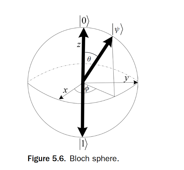
A generic qubit is of the form

$$|\psi\rangle = c_0|0\rangle + c_1|1\rangle$$

where $|c_0|^2 + |c_1|^2 = 1$. The equation can be written as:

$$|\psi\rangle = \cos(\theta)|0\rangle + e^{i\phi}\sin(\theta)|1\rangle$$

with only two parameters $\theta$ and $\phi$ to describe the state.

• A phase shift gate is defined as

$$R(\theta) = \begin{bmatrix} 1 & 0 \\ 0 & e^{i\theta} \end{bmatrix}$$

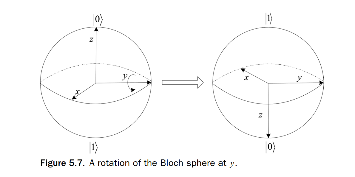
• Sometimes we want to rorate a particular number of degrees around the x,y or z axis, which can be represented as:

$$R_x(\theta) = \cos{\frac{\theta}{2} I} - i \sin{\frac{\theta}{2}X} = \begin{bmatrix} \cos{\frac{\theta}{2}} & -i \sin{\frac{\theta}{2}} \\ - i \sin{\frac{\theta}{2}} & \cos{\frac{\theta}{2}} \end{bmatrix}$$ $$R_y(\theta) = \cos{\frac{\theta}{2} I} - i \sin{\frac{\theta}{2}Y} = \begin{bmatrix} \cos{\frac{\theta}{2}} & - \sin{\frac{\theta}{2}} \\ \sin{\frac{\theta}{2}} & \cos{\frac{\theta}{2}} \end{bmatrix}$$ $$R_z(\theta) = \cos{\frac{\theta}{2} I} - i \sin{\frac{\theta}{2}Z} = \begin{bmatrix} e^{-i\theta/2} & 0 \\ 0 & e^{i\theta/2} \end{bmatrix}$$

Basic Quantum Mechanics

The time evoluation of the state of a closed quantum system is described by the Schrödinger equation:

$$i\hbar \frac{d|\psi\rangle}{dt} = H|\psi\rangle$$

$\hbar$ is a physical constant known as Planck's constant whose value must be experimentally determined.

where $H$ is the Hamiltonian of the system.

Density matrix Density matrix or density operator ($\rho$) is an alternative formulation for state vectors.

• The trace of a density matrix $tr(\rho) = 1$.

The evolution of a closed quantum system is described by a unitary transformation.That is, the state $\rho$ of the system at time $t_1$ is related to the state $\rho'$ of the system at time $t_2$ by a unitary operator $U$ which depends only on the time $t_1$ and $t_2$

$$\rho' = U\rho U^{\dagger}$$

A pure state satisfied $Tr(\rho^2) = 1$
For a mixed state, $Tr(\rho^2) < 1$

For pure state: rank = 1, $det(\rho) = \lambda_1 \lambda_2 = 0$

Calculation tricks

Complex Conjugate of a matrix

$$A = \begin{bmatrix} 1+i & 2-3i \\ 4 & 5i\end{bmatrix} \quad A^{\dagger} = \begin{bmatrix} 1- i & 4 \\ 2 + 3i & -5i\end{bmatrix}$$

Trace of a matrix

$$A = \begin{bmatrix} a_{11} & a_{12} \\ a_{21} & a_{22}\end{bmatrix} \quad \text{tr}(A) = \sum_{i = 1}^3 a_{ii} = a_{11} + a_{22}$$

Transformation of complex number

Regular form:

$$z=x+iy$$

Polar Form:

$$r = |z| = \sqrt{x^2 + y^2} \\[5pt] \theta = arg(z) = tan^{-1} (\frac{y}{x}) \\[5pt] \bf{z = r(\cos{\theta} + i \sin{\theta})} \quad \leftarrow \text{final form}$$

Exponential Form:
Euler's formula : $e^{i \theta} = \cos{\theta} + i \sin{\theta}$

Thus the exponential form:

$$z = r e^{i \theta}$$

Matric multipliation

$$A = \begin{bmatrix} a & b \\ c & d\end{bmatrix} \quad B = \begin{bmatrix} e & f \\ g & h\end{bmatrix} \\[6pt] A \times B = \begin{bmatrix} a×e+b×g & a×f+b×h \\ c×e+d×g & c×f+d×h \end{bmatrix}$$

Some normal gate combination

$$X^2 = Y^2 = Z^2 = I \\ H = \frac{1}{\sqrt{2}}(X+Z)\\ X = HZH \quad Z = HXH \quad -1Y = HYH \\ S = T^2 \\ -1Y = XYX$$

Embedding Data

Basis Embedding

$$b = (b_0, b_1, ..., b_{n-1}) \rightarrow |b_0, b_1, \ldots, b_{n-1}\rangle$$

Pros:

• Simple and intuitive: It directly maps binary data into quantum states, making it suitable for data that is inherently binary.

Cons:

• High resource consumption: If the input data is not binary, it needs to be converted before encoding. Each bit requires one qubit, leading to high resource consumption, especially for large datasets.

Angle Embedding

Angle embedding is suitable for floating-point data.

It encodes each input value 𝑥 as a rotation around one of the axes (𝑥,𝑦,𝑧) on the Bloch sphere

$$x \mapsto R_k(x) \lvert 0 \rangle = e^{-i \frac{x}{2} \sigma_k} \lvert 0 \rangle,$$

Pros:

• Fewer qubit requirements: Each feature can be encoded using a rotation gate, which saves qubit resources.
• Ideal for continuous data: It works well for handling floating-point or other continuous data.

Cons:

• Non-unique mapping: Different data may be mapped to the same quantum state since the same rotation angle can result in identical quantum states.
• Initial state limitation: If the initial state is $|0\rangle$, rotations around the z-axis have no effect, making them unusable for encoding in such cases.

Amplitude Embedding Amplitude embedding encodes the values of an input array as the amplitudes of a quantum state. Specifically, the input $a = (a_0, a_1, ..., a_{2^n-1})$ is encoded as:

$$|a\rangle = \sum_{i=0}^{2^n-1} a_i |i\rangle$$

requiring that the amplitudes are normalized, i.e. $\|a_i\| = 1$.

Pros:

• Efficient qubit usage: It can represent a large amount of data in a single quantum state, particularly suitable for large-scale data where an exponential number of data points can be represented.
• High representational capacity: It allows data to be embedded into high-dimensional quantum states, enabling quantum machine learning models to learn complex features in higher-dimensional space.

Cons:

• Normalization requirement: Input data must be normalized to ensure that all the squared amplitudes sum to 1, which can add computational complexity.

• Complex circuit design: Implementing amplitude embedding requires complex multi-controlled rotations, making the circuit design and implementation more challenging.