Cross validation

Compare different algorithms in terms of performance from limited available data and help choose hyperparameters for an algorithm

Performance matrices

• Given a dataset $D = \{x_1, y_1, \ldots, x_n, y_n \}$ of n samples.
• For a data point $x_i$ we predict $g(x_i)$

Matrices in regression

• Mean squared error: $MSE(g) = \frac{1}{n} \sum_{i = 1}^{n}(g(x_i)-y_i)^2$
• Root mean squared error: $RMSE(g) = \sqrt{MSE(g)}$
• Mean absolute error: $\frac{1}{n}\sum_{i=1}^{n} |g(x_i)-y_i|$

Performance metrics in classification

	True Label +1	True Label -1
Predicted +1	TP	FP
Predicted -1	FN	TN

• Accurcy: (𝑇𝑃 + 𝑇𝑁) / (𝑇𝑃 + 𝐹𝑃 + 𝐹𝑁 + 𝑇𝑁)
• Error: (𝐹𝑃 + 𝐹𝑁)/(𝑇𝑃 + 𝐹𝑃 + 𝐹𝑁 + 𝑇𝑁)
• Recall/Sensitivity: 𝑇𝑃/(𝑇𝑃 + 𝐹𝑁)
• Precision 𝑇𝑃/(𝑇𝑃 + 𝐹𝑃)
• Specificity 𝑇𝑁/(𝑇𝑁 + 𝐹𝑃)
• F1-score: 2 𝑃𝑟𝑒𝑐𝑖𝑠𝑖𝑜𝑛 × 𝑅𝑒𝑐𝑎𝑙𝑙/(𝑃𝑟𝑒𝑐𝑖𝑠𝑖𝑜𝑛 + 𝑅𝑒𝑐𝑎𝑙𝑙)

Receiver Operating Characteristic (ROC)

Summarized with an Area Under the Curve (AUC):

• Random: 0.5
• Perfect Classifier: 1

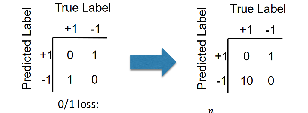
Modified loss function

Different misclassification have difference influence

Predicting a diseased patient as healthy has much worse serious consequences than predicting a diseased patient as healthy!!!

Cross-validation: using “unseen” data

Split datasets in three parts

Training Set	Validation Set	Test Set

K-Fold Cross Validation

• Split training data $D$ into $k$ disjoint sets $S_1, \ldots, S_k$
  • Either randomly, or in a fixed fashion
  • If $D$ has $n$ samples, then each fold has approximately $\frac{n}{k}$ samples
  • Popular choices: $k = 5, k = 10, k = n$ (leave one out)
• For $i = 1 \ldots k$
  • train with sets $S_1, \ldots, S_{i-1}, S_{i+1},\ldots, S_k$
  • test on set $S_i$
  • let $M_i$ be the test metric (e.g., accuracy, MSE)

Mean $\hat{u} = \sum_{i = 1}^{k}\quad$ variance $\hat{\sigma}^2 = \sum_{i = 1}^{k} (M_i - \hat{u})^2$

0.632 Bootstrapping

Let $B > 0$, and $n$ be the number of training samples in $D$

• For $i = 1 \ldots B$ :
  • Pick n samples from $D$ with replacment, call it $S_i$ ($S_i$ might contain the same sample more than once)
  • train with set $S_i$
  • test on the remaining samples $(D - S_i)$
  • let $M_i$ be the test metric (e.g., accuracy, MSE)

Mean $\hat{u} = \sum_{i = 1}^{B} M_i \quad$ variance $\hat{\sigma}^2 = \sum_{i = 1}^{k} (M_i - \hat{u})^2$

• not picking one particular item in 1 draw is 1 − 1/𝑛
• not picking one particular item in 𝑛 draws is $(1 − 1/𝑛)^2$
• picking one particular item in 𝑛 draws is $1- (1 − 1/𝑛)^2$

Finally: $\lim_{n\to\infty} 1-(1-1/n)^n = 1-1/e \approx 0.632$

Nested Cross-valdation

• Useful for hyperparameter tuning
• Inner cross-vaildation (e.g., 0.632 bootstapping) to try different hypermarameters
• Outer cross-validation (e.g., k-folds) to report metric using the best hyptermenter

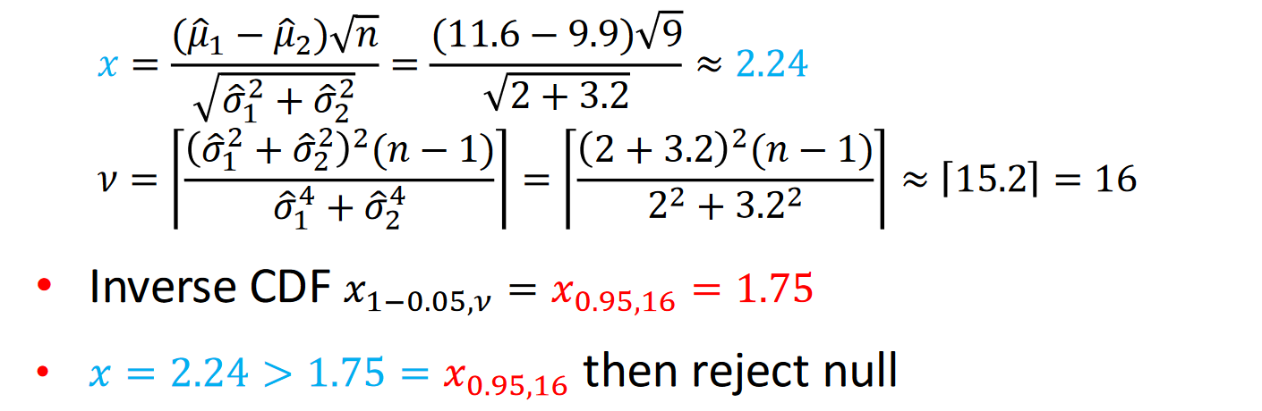
Hypothesis testing

• Let $\hat{u_1},\hat{u_2},\hat{\sigma_1}^2,\hat{\sigma_2}^2$ be mean and variance of algorithms 1 and 2

$$\text{Let} \, x = \frac{(\hat{\mu}_1-\hat{\mu}_2)\sqrt{n}}{\sqrt{\hat{\sigma}_1^2+\hat{\sigma}_2^2}} \qquad \nu = \left\lfloor\frac{(\hat{\sigma}_1^2+\hat{\sigma}_2^2)^2(n-1)}{\hat{\sigma}_1^4+\hat{\sigma}_2^4}\right\rfloor$$

v using upper bound, degrees of freedom of Student's t-distribution

Examples

Learning with expert advice

In machine learning, the term "expert" typically refers to a model or algorithm with specialized knowledge or predictive ability for a specific task or domain.

Learning from expert advice

• Learner listens to some / all experts making decisions
• True outcomes are ADVERSARIAL
• Learner updates weights over experts based on their loses
• Algorithm all forms of "multiplicative weights"
• Nice clean bounds on total mistakes/losses: by "potential function" technique

Adversarial

• The real outcomes do not come from a fixed probability distribution, but rather may be chosen by an adversary attempting to make the learner fail. This is a conservative assumption that ensures the algorithm performs well even in worst-case scenarios. Under this setting, algorithms need to be adversarial, capable of handling the most unfavorable situations. potential function and clean upper bound Using potential functions, we can derive explicit upper bounds on the algorithm's cumulative number of mistakes or total loss.

Infallible expert(one always perfect)

• Majority Vote Algorithm

Imperfect experts(none guaranteed perfect)-incresingly better

• Weighted Majority Vote Algorithm by Halving
• Weighted Majority Voting by General Multiplicative Weights
• Probabilistic Experts Algorithm

Infallible Expert Algorithm: Majority Vote

1. Initialzie set of experts who haven't made any mistakes
2. Repeat per round
   • Observe perdictions E_i for all $i \in \{1, \ldots, n\}$
   • Make majority prediction $\argmax_{y \in \{-1,1\}} \sum_{i \in E} 1[E_i = y]$
   • Overve correct outcome
   • Remove mistaken experts from E

Mistake bound for Majority Vote Under infallible expert assumption, majiroty vote makes total misktakes $M \leq \log_2 n$

Imperfect experts and the Halving Algorithm

No more guarantee of an infallible expert

“Zero tolerance” dropping experts on a mistake is No sense

Imperfect experts: Halving Algorithm

1. Initialize $w_i = 1$ weight of expert $E_i$
2. Repeat per round
   • Observe predicitions $E_i$ for all $i \in \{1, \ldots, n\}$
   • Make weighted majority prediction $\argmax_{y \in \{-1,1\}} \sum_{i \in E} w_i 1[E_i = y]$
   • Oberve correct outcome
   • Downweigh each mistaken expert $E_i \quad w_i \leftarrow w_i / 2$

Mistake bound for Halving
If the best expert makes m mistakes, then weighted majority vote makes $M \leq 2.4(m + \log_2 n)$ mistakes

From Halving to Multiply weights by $1- \epsilon$

1. Initialize $w_i = 1$ weight of expert $E_i$
2. Repeat per round
   • Observe predicitions $E_i$ for all $i \in \{1, \ldots, n\}$
   • Make weighted majority prediction $\argmax_{y \in \{-1,1\}} \sum_{i \in E} w_i 1[E_i = y]$
   • Oberve correct outcome
   • Downweigh each mistaken expert $E_i \quad w_i \leftarrow w_i (1- \epsilon)$

Mistaken bound for $1- \epsilon$
If the best expert makes $m$ mistakes, then $1-\epsilon$ weighted majority vote makes $M \leq 2(1+ \epsilon)m + (2\log_e n) /\epsilon$ mistakes

Mini Conclusion

In the case of imperfect experts, the number of mistakes made by the weighted majority algorithm depends on the number of mistakes made by the best expert 𝑚, and the coefficient 2 in this dependency relationship is unavoidable.

The probabilistic experts algorithm

• Change 1: change from mistakes to loss: $\text{Loss} \ell_i^{(t)} \in [0,1]$ of $E_i$
• Change 2: Randomised algorithm means, bounding expected losses (It is a risk!)

1. Initialize $w_i = 1$ weight of expert $E_i$
2. Repeat per round
   • Oberve predicitons $E_i$ for all $i \in \{1, \ldots, n\}$
   • Predict $E_i$ of expert i with probability $\frac{w_i}{W}$ where $W = \sum_{j=1}^{n} w_j$
   • Observe losses
   • Update each weight $w_i \leftarrow (1-\epsilon)^{\ell_i^{(t)}} w_i$

Expected loss bound
Expected loss of probalistic expert alghorithm is $L \leq \frac{\log n }{\epsilon} + (1 + \epsilon)L^*$ where $L^*$ is the minimum loss over experts

MAB

Where we learn to take actions; we receive only indirect supervision in the form of rewards

Multi-Armed Bandit

• Simplest setting for balancing exploration, exploitation
• Same familiy of ML tasks as reinforcement learning

Stochastic MAB setting

Possible actions $\{ 1,\ldots, k \}$ called "arms"

• Arm i has distributon $Pi$ on bounded rewards with mean $\mu_i$

In round $t = 1, \ldots, T$:

• Play action $i_t \in \{1, \ldots, k\}$
• Receive reward $R_{i_t}(t) \sim p_{i_t}$

Goal: minimize cumlative regret

• $u^* T - \sum_{t=1}^{T} E[R_{i_t}(t)]$ where $u^* = \max_i u_i$

Greedy

At round t,

• Estimate value of each arm i as average reward observed

$$Q_{t-1}(i) = \begin{cases} \frac{\sum_{s=1}^{t-1} R_i(s) \mathbb{1}[i_s = i]}{\sum_{s=1}^{t-1} \mathbb{1}[i_s = i]}, & \text{if } \sum_{s=1}^{t-1} \mathbb{1}[I_s = i] > 0 \\ Q_0, & \text{otherwise} \end{cases}$$

Some init constant $Q_0(i) = Q_0$ used until arm i has been puolled

Eploit! $i_t \in \argmax_{1\leq i \leq k} Q_{t-1}(i)$

$\epsilon$ - Greedy

At round t

• Estimate value of each arm $i$ as average reward observed (Q- value function is same as greedy)

$$Q_{t-1}(i) = \begin{cases} \frac{\sum_{s=1}^{t-1} R_i(s) \mathbb{1}[i_s = i]}{\sum_{s=1}^{t-1} \mathbb{1}[i_s = i]}, & \text{if } \sum_{s=1}^{t-1} \mathbb{1}[I_s = i] > 0 \\ Q_0, & \text{otherwise} \end{cases}$$

Exloit:

$$i_t \sim \begin{cases} \arg \max_{1 \leq i \leq k} Q_{t-1}(i), & \text{with probability } 1 - \epsilon \\ \text{Unif}(\{1, \ldots, k\}), & \text{with probability } \epsilon \end{cases}$$

$\epsilon$ controls exploration vs. exploitation

• Larger $\epsilon$ will increase the change to exploration
• Smaller $\epsilon$ will tend to choose exploitation

Upper-Confidence Bound (UCB)

$$Q_{t-1}(i) = \begin{cases} \hat{\mu}_{t-1}(i) + \sqrt{\frac{2 \log(t)}{N_{t-1}(i)}}, & \text{if } \sum_{s=1}^{t-1} \mathbb{1}[I_s = i] > 0 \\ Q_0, & \text{otherwise} \end{cases}$$

Some init constant $Q_0(i) = Q_0$ used until arm i has been puolled

$$N_{t-1}(i) = \sum_{s=1}^{t-1} \mathbb{1}[I_s = i] \quad \hat{\mu}_{t-1}(i) = \frac{\sum_{s=1}^{t-1} R_i(s) \mathbb{1}[I_s = i]}{\sum_{s=1}^{t-1} \mathbb{1}[I_s = i]}$$