From lec2 to lec5

Linear Regression

Model: $H = a + bT$

• Criterion: minimise the sum of squared errors

Expressed as matrix form:

$$y = X\beta + \epsilon$$

where $\epsilon \sim \mathcal{N}(0, \sigma^2)$
thus $y \sim \mathcal{N}(x'w , \epsilon)$

Maximum-likelihood estimation: Choose parameter values that maximise the probability of observed data

$$p(y_1, ..., y_n|x_1, ..., x_n) = \prod_{i=1}^n p(y_i|x_i)$$

Maximising log-likelihood as a function of 𝒘 is equivalent to minimising the sum of squared errors

$$L = y'y - 2y'Xw + wX'Xw$$

Solving for 𝒘 yields:

$$\hat{w} = (X^T X)^{-1} X^T y$$

$𝑿'$ denotes transpose
$X'X$ should be an invertible matrix, that is: a full rank matrix, column vectorsw linear independence

Basis expansion for linear regression: Turn linear regression to polynomial regression for better fit the data

Logistic regression

Logistic regression assumes a Bernoulli distribution with parameter
and is a model for solving binary classification problems

$$P(Y=1|\mathbf{x}) = \frac{1}{1 + \exp(-\mathbf{x}'w)}$$

MLE for Logistic regression cannot get an analytical solution.

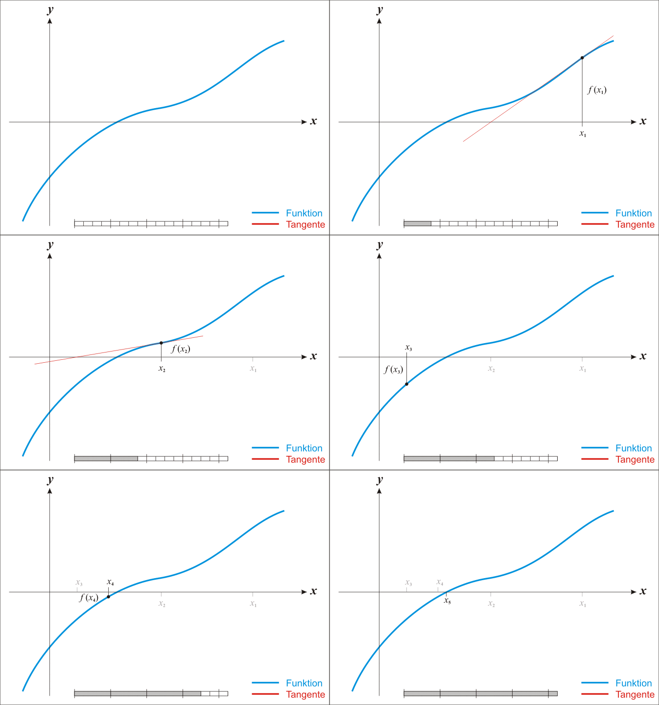
We introduce: Approximate iterative solution

• Stochastic Gradient Descent (SGD)
• Newton-Raphson Method

Stochastic Gradient Descent (SGD)

Newton-Raphson Method

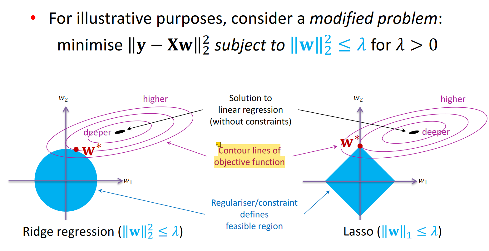
Regularization

Normal equations solution of linear regression:

$$\hat{w} = (X^T X)^{-1} X^T y$$

With irrelevant/multicolinear features, matrix 𝐗!𝐗 has no inverseRegularisation: introduce an additional condition into the system

$$\|y - Xw\|_2^2 + \lambda\|w\|_2^2 \text{ for } \lambda > 0$$

Adds 𝜆 to eigenvalues of $𝐗'𝐗$: makes invertible : ridge regression

Lasso (L1 regularisation) encourages solutions to sit on the axes
Some of the weights are set to zero $\rightarrow$ Solution is sparse